Scientific Computing in Rust

While getting my degree in Physics, I had to take classes in both MatLab and Python for scientific computing. I preferred python, where we used the SciPy and NumPy packages. In fact, I used those packages again (along with matplotlib) in an undergraduate research project simulating bacteria films. There’s a catch: I was also pursuing a degree in Computer Science, and Python just wasn’t fast enough for that side of me, so, during my free time in graduate school, I rewrote my biofilm simulation in my new favorite language, Rust.

First problem: I needed to replace jsonpickle for data serialization. This problem was easy, as the serde crate is an amazing replacement (I even transitioned from JSON to Rusty Object Notation, RON). Second problem: Should I try to get matplotlib bindings in Rust or should I use a more Rust-y plotting library? I decided on the latter, finding plotters to be a suitable replacement for matplotlib. Last problem: How do I replace the differential equation solvers of SciPy? I ended up writing a custom predictor-corrector solver which worked well enough, giving identical simulation results while being five hundred times faster than my python code at just the simulation step, rendering not included (plotting directly to an RGB buffer then using libx264 bindings to generate raw H.264 frames that mpv can understand also gave a similar speedup to the rendering step over writing out every frame as a png file in matplotlib and using a shell script to ffmpeg the outputs together). Full disclosure, a large part of this speedup probably comes from my derivative function being not-python, rather than my implementation of a differential equation solver over SciPy’s. Furthermore, I only breached the five hundred barrier when switching to using a QuadTree to find the nearest neighbors of a bacteria, before that the speed up was more in the three hundreds. This port of my old project can be found here if you care for some reason.

Introducing bacon-sci

Inspired, I decided to start on a full SciPy replacement in rust as I could not find one I liked on crates.io (I later found the peroxide crate). I even had a clever name: bacon, named after Francis Bacon and the pork based food; however, bacon is already a crate, so I went for the next best thing: bacon-sci.

I started out with the easiest part. SciPy has a set of scientific constants from the NIST. I just took the list of important constants from SciPy and put it in a module. In addition, I took NIST’s CODATA and put it into a global map that corresponds a String of the constant’s name to a triplet: an f64 of its value, an f64 of its uncertainty, and a String of its units. How do you make a static map? I just used the lazy_static crate.

Next, I returned to the area that inspired me: initial value problems. After that, I tackled root finding and polynomials. Lastly, as of now, I implemented a few special polynomials and numeric differentiation. Armed with a copy of Burden and Faires’s “Numerical Analysis (8th ed.)”, Wikipedia, and SciPy source code, I went to work.

The first decision I made was to use a linear algebra crate, specifically nalgebra. I have written many vector and matrix implementations in the past, and I didn’t feel like doing it this time. Besides, nalgebra is probably faster than anything I can write.

The next decision was using the alga crate to handle generics of complex types and real types. I wanted all algorithms that could work on complex numbers to be able to, so most of the functions in bacon-sci work on N: ComplexField. If an algorithm requires a parameter to be well-ordered (like time), then it is a N: RealField. In cases where a function takes both, the generic parameter is a N: ComplexField with the real parameters being N::RealField, which is the real “backing type” of the possibly complex field. Some functions require complex arithmetic, so they automatically upgrade from N: ComplexField to Complex<N::RealField> from num_complex.

Interestingly, there are cases where I wanted to automatically downgrade from definitely complex back to “maybe complex”, which was more difficult than the other way. To upgrade, all I needed was Complex::<N::RealField>::new(z.real(), z.imaginary()), where z is a possibly complex value, with real types giving zero on the imaginary component. To go the other way, I decided to basically take the real component and ignore the imaginary component. To do this from a N: ComplexField I had to check if N::RealField == N to see if N was real or complex. To do this, I used TypeId::of::<N::RealField>() == TypeId::of::<N>(). If N was real, converting from complex was easy: use ComplexField::from_real on the real component, ignoring the imaginary. On the other hand, if N was complex, the conversion needed to preserve the imaginary component. ComplexField has no from_imaginary, so I directly implemented $a + bi$ with ComplexField::from_real(z.re) + (-ComplexField::one()).sqrt() * ComplexField::from_real(z.im), with z being the definitely complex value.

Euler Method

A differential equation is an equation describing a thing in terms of how that thing changes. For those unfamiliar, this is a good introduction. In order to solve a differential equation, you need some conditions. These come in two flavors: boundary conditions and initial values, with both names being self-describing. My second task on bacon-sci was to implement algorithms that solve initial value differential equations, referred to as initial value problems or ivp in the code.

Abstractly, the system of differential equations can be written, with an arrow representing a vector quantity, as $$\frac{\mathrm{d}\vec{y}}{\mathrm{d}t} = f(t, \vec{y}) .$$ This is a first-order system of differential equations since only the first derivative is present. Generally, many higher-order equations can be reduced to first-order by thinking of each derivative as a new variable. The initial condition is then represented as $$\vec{y}(t_0) = \vec{y}_0$$

These equations immediately lead to the first algorithm for solving initial value problems, Euler’s method. Consider this question: given a time-step $\Delta t$ , what is the corresponding $\Delta \vec{y}$ ? We can approximate $\Delta \vec{y} / \Delta t \approx \mathrm{d}\vec{y}/\mathrm{d}t = f(t, \vec{y})$ , (that is, use the tangent line to estimate the function), leading to $\Delta \vec{y} = f(t, \vec{y} )\Delta t$ . This gives us an iterative algorithm, $\vec{y}_{i + 1} = \vec{y}_{i} + f(t, \vec{y})\Delta t$ . This is Euler’s method. From the starting conditions, pick a time-step and iterate until you reach the end.

So how good is Euler’s method? Not very good. As an example, imagine solving a mechanics differential equation with positions and velocities. Conservation of energy says that energy should be conserved. Will Euler’s method conserve energy? In general, it will not. Energy in Euler’s method tends to explode. One solution to this is to use a slightly different version of the algorithm known as Euler-Cromer or the semi-implicit Euler’s method. In this method, velocities are updated first, then positions are updated using the new velocities (in Euler’s method, you’d use the old velocities). Euler-Cromer is much better, tending to conserve energy, especially in spring systems. According to Gaffer on Games, game physics tend to use the Euler-Cromer as it only requires calculating the derivative once but gives much better results than Euler’s.

Runge-Kutta Methods

One problem with Euler’s method is that the error in each step is linear in the step size. We can do better. To start with, remember Taylor series from basic calculus. That is, remember you can approximate a function of one variable like $$f(x) = f(x_0) + f'(x_0) (x - x_0) + \frac{f''(x_0)}{2} {(x - x_0)}^2 + \ldots .$$ Similarly, we can approximate our derivative function from the last section with $$f(t, \vec{y}) = f(t_0, \vec{y}_0) + \left((t - t_0)\frac{\partial f}{\partial t}(t_0, \vec{y}_0) +(\vec{y} - \vec{y}_0)\frac{\partial f}{\partial \vec{y}}(t_0, \vec{y}_0)\right) + \ldots ,$$ where the powers of our vectors are done element-wise. Additionally, Taylor’s Theorem bounds the error via some small parameters $\xi, \mu$ . In this light, we can say Euler’s method is a zeroth order approximation, which is why the error is linear. You can use Taylor polynomials for better IVP solvers, but this requires information about the derivatives of $f$ . Instead, Runge-Kutta methods allow for tighter error bounds without using the derivative.

To see an example of this, I will derive the midpoint method here. Imagine for a moment that instead of taking a full time-step, you take a partial time-step and use $f$ at that point to approximate the second Taylor polynomial. That is, choose a $a_1, \alpha_1, \beta_1$ so that $a_1 f(t + \alpha_1, \vec{y} + \beta_1)$ approximates $$T^{(2)}(t, \vec{y}) = f(t, \vec{y}) + \frac{h}{2}f'(t, \vec{y}),$$ where $h$ is the time-step, with quadratic error in the time-step. Note that $f'(t, y) = \partial f/\partial t(t, \vec{y}) + \partial f/\partial \vec{y}(t, \vec{y}) \vec{y}'(t)$ . Thus, $$T^{(2)} = f(t, \vec{y}) + \frac{h}{2}\frac{\partial f}{\partial t}f(t, \vec{y}) + \frac{h}{2}\frac{\partial f}{\partial \vec{y}}(t, \vec{y}) f(t, \vec{y}) .$$ Expanding $a_1 f(t + \alpha_1, \vec{y} + \beta_1)$ via Taylor series gives $$a_1 f(t, \vec{y}) + a_1 \alpha_1 \frac{\partial f}{\partial t}(t, \vec{y}) + a_1\beta_1 \frac{\partial f}{\partial y}(t, y) .$$ Thus, $a_1 = 1$ , $a_1 \alpha_1 = h/2$ , and $a_1 \beta_1 = f(t, \vec{y}) h / 2$ . This uniquely determines the coefficients, giving rise to the midpoint method: $$\vec{y}_{i + 1} = \vec{y}_i + hf\left(t_i + \frac{h}{2}, \vec{y}_i + \frac{h}{2}f\left(t_i, \vec{y}_i\right)\right) .$$

This process can be repeated for higher order polynomials. The classic Runge-Kutta method is order 4, and is used as follows: $$\vec{k}_1 = hf(t_i, \vec{y}_i),$$ $$\vec{k}_2 = hf\left(t_i + \frac{h}{2}, \vec{y}_i + \frac{1}{2}\vec{k}_1\right),$$ $$\vec{k}_3 = hf\left(t_i + \frac{h}{2}, \vec{y}_i + \frac{1}{2}\vec{k}_2\right),$$ $$\vec{k}_4 = hf(t_i + h, \vec{y}_i + \vec{k}_3),$$ $$\vec{y}_{i+1} = \vec{y}_i + \frac{1}{6}(\vec{k}_1 + 2\vec{k}_2 + 2\vec{k}_3 + \vec{k}_4).$$ This is almost what is in bacon-sci. Note that Runge-Kutta methods can be described by a table of the coefficients of $h$ when added to $t_i$ for the various intermediate steps, the coefficients of each previous intermediate step for an intermediate step, and the final weighted average coefficients.

Adam-Bashforth Methods

There’s a problem with all the IVP solvers discussed so far. The algorithm may take steps between two solution points, but it never remembers those steps. In other words, we throw away a lot of useful information. Multistep methods solve this problem by retaining information about previous steps. In an equation, you can characterize an $m$ step method as $$\vec{y}_{i+1} = \sum_{j=0}^{m-1} a_{m-1-j}\vec{y}_{i-j} + h\sum_{j=0}^{m} b_j f(t_{i+1-m + j}).$$ Notice that some methods can have a point depend on the derivative at that point. These are implicit methods.

Adam-Bashforth methods are explicit methods that use Newton’s backward difference formula to find the coefficients. bacon-sci almost implements a fifth order Adams-Bashforth method.

Adaptive Step Size Methods

Still, all of these methods have a problem. The step size, $h$ , is the same for complicated interesting parts of the solution and boring flat parts! Ideally, the step size will be small in the complex bits and large in the flat bits to minimize computation time. Enter adaptive step size methods!

The main idea of adaptive step sizes is to have two estimates of the next step, one more accurate and one less accurate. Let the norm of the difference between the two be the error. If the error is small, then increase the step size. If the error is large, try the step again with a smaller step size. A simple algorithm for any of the above solvers is to solve the next step twice, once with the full step size and once with half the step size. Then, if the error is too small, double the step size. If the error is too big, half the step size. This algorithm works, but is computationally expensive, and smaller step sizes may produce worse results due to round-off error. Better methods exist.

A good way to estimate error for Runge-Kutta methods is to use two orders of methods, taking the value from the higher order method. The classic example of this is the Runge-Kutta-Fehlberg method, which uses an order 4 and order 5 method. The best part about this technique is that the fourth and fifth order methods share some intermediate steps, so only 6 intermediate steps need to be found!

For the multistep solvers, a good strategy is to make a prediction of the next step using an explicit method. Then, take the prediction and use it in an implicit method of the same order. These techniques are known as predictor-corrector methods.

Finally, I can talk about the implementation of bacon-sci. In my crate, I have a trait IVPSolver that defines everything I want an IVPSolver to be. The trait specifies a builder-style API for making a solver, giving a method to turn the solver into a normal rust iterator at the end (plus a convienence function for collecting into a result containing a vector). I have one direct implementation, Euler. On top of that, I have Adams, BDF, and RungeKutta structs implement IVPSolver based on a generic parameter defining the order of the method. This is possible since each class of method uses the same algorithm, regardless of order, just with different constants. Thus, I have the traits AdamsCoefficients, etc., that specify which constants are needed for each method, and type aliases for the main solving structs that fill out the required generic parameter. This means the user will be able to use Adams5 to get an Adams struct filled with the correct 5th-order constants, making it easy to use and making development easier, too!

What else is there for bacon-sci? Well, there exist methods known an backwards differentiation formulas which are very useful for differential equations the aforementioned methods fail at; however, they are implicit methods. How does one solve an implicit equation? Well, stay tuned!

Solving Initial Value Problems with bacon-sci

The theory is all well and good, but how do you solve an initial value problem with bacon-sci? There are currently seven implemented solvers in the library: RungeKutta45, RungeKutta23, Adams5, Adams2, BDF6, BDF2, and Euler. As mentioned previously, IVPSolver is a trait, so all of these solvers have a shared interface. For this example, I’ll solve a one-dimensional problem with $y(0) = 0$ using RungeKutta45. The derivative function (that is, $f(t, y)$ is of the form: fn deriv<T>(t: f64, y: &[f64], params: &mut T) -> Result<SVector<f64, 1>, Box<dyn Error>> { ... }. Here, I am using f64 for both t and y, but f32 would work as well (you can even have y be a Complex<{float}> type with t being the corresponding real float type). In this case, you’d solve the initial value problem in a manner such as:

fn solve() -> Result<SVector<f64, 1>, IVPError> {
    let mut rk = RungeKutta45::new()
        .with_minimum_dt(0.01)?
        .with_maximum_dt(0.1)?
        .with_tolerance(1e-3)?
        .with_initial_time(0.0)?
        .with_ending_time(1.0)?
        .with_initial_conditions_slice(&[1.0])?
        .with_derivative(deriv)
        .solve(())?;

    rk.collect_vec()
}

Root finding

After initial value problems, the next area of numerical analysis I tackled is root finding. What is root finding? It’s finding the solutions of $$f(x) = 0,$$ for an arbitrary function. In other words, you are finding where a function becomes zero. There’s a related problem of finding stationary points, that is the solutions of $$f(x) = x,$$ for an arbitrary function. Problems can be easily translated between the two domains; however, in bacon-sci I have only implemented algorithms for the first problem, root finding.

What are the algorithms bacon-sci has? I have currently implemented the bisection method, Newton’s method, the secant method, and Müller’s method for polynomials.

Bisection Method

The bisection method is the easiest to understand. It requires two starting points, $a$ and $b$ , such that the sign of $f(a)$ and the sign of $f(b)$ are different (if one is zero then you found a root!). Then, the algorithm performs a binary search, dividing the interval $[a,b]$ in half. At the midpoint, the sign of the function is either zero, meaning success, the same as at $a$ or the same as at $b$ . Thusly, you either get a result or have one new interval with differing signs at the end points. This is done recursively until an answer is found.

What are the problems with this method? Firstly, you need two starting points with differing signs. Next, this only works with single dimensional real numbers. Other algorithms described here work with complex vector functions. On the bright side, the initial two guesses can be any distance from a root of the function without the algorithm failing. I should note here that there’s a closely related algorithm called the method of false position. In this algorithm, instead of the midpoint, you choose the dividing line between two subintervals to be where the line from $f(a)$ to $f(b)$ crosses the x axis.

The bisection method is implemented as bacon_sci::roots::bisection.

Newton’s Method

Newton’s method is a more sophisticated method of root finding. To derive it, first assume that $f$ is continuous and doubly differentiable on $[a,b]$ . Now, give a starting guess for the root, $p_0$ . Then, we can expand $f$ as a Taylor series centered at $p_0$ : $$f(p) = f(p_0) + (p - p_0)f'(p_0) + \ldots .$$ Ignoring the higher order terms, $$f(p) = f(p_0) + (p - p_0)f'(p_0) .$$ Now, let $p$ be the true root of the function. Thus, $$0 = f(p_0) + (p - p_0)f'(p_0) ,$$ $$0 = f(p_0) + pf'(p_0) - p_0f'(p_0),$$ $$pf'(p_0) = p_0 f'(p_0) - f(p_0),$$ $$p = p_0 - \frac{f(p_0)}{f'(p_0)}.$$ Since we ignored higher order terms, this is only an approximation of the true root $p$ . However, this is a better approximation than the starting one!

Iterating this equation over and over again until the guess produces a zero of the function is Newton’s method. What are the problems with it? Firstly, there’s the obvious problem that you need the derivative of the function, which may not be available. Secondly, the procedure fails if the derivative is ever zero. Thirdly, the process fails if the initial guess is far from a root (Taylor series need only be accurate around the point of expansion).

Newton’s method is implemented as bacon_sci::roots::newton, with a specialized version for polynomials as bacon_sci::roots::newton_polynomial.

Secant Method

The secant method is an adaptation of Newton’s method to remove the need for an explicit derivative. To derive it, imagine calculating $p_{n+1}$ , the $n+1$ th iteration of Newton’s method. You would need the derivative at $p_n$ , but the derivative at that point is just the slope of the tangent line at that point! This can be approximated by a secant line from the point and a nearby point. Luckily, we have a nearby point: $p_{n-1}$ . Thus, $$f'(p_n) \approx \frac{f(p_n) - f(p_{n-1})}{p_n - p_{n-1}} .$$ Putting this into Newton’s method, $$p_{n+1} = p_n + \frac{f(p_n)(p_n - p_{n-1})}{f(p_n) - f(p_{n-1})} .$$ This is the secant method.

The secant method has an obvious advantage over Newton’s method. It also has an obvious trade-off: you need two starting points instead of one. There is also a trade-off that the secant method shares with Newton’s method: the roots aren’t bracketed. What does this mean? In the bisection method, we always had an interval within which there was sure to be a root. The root we were approaching always was within this interval. The successive iterations of Newton’s method and the secant method do not bracket a root like this. There is a second method of false position which modifies the secant method to be bracketed, but bacon-sci does not implement either version.

The secant method is implemented as bacon_sci::roots::secant.

Müller’s Method

Müller’s method is related to the secant method. While the secant method uses a line to approximate the derivative, Müller’s method uses a parabola. Currently, bacon-sci only implements Müller’s method for polynomials.

This concludes a tour of the root finding available in bacon-sci. I think these methods are rather out of date, especially for polynomial root finding. In the case of polynomials, I solve for linear and quadratic roots exactly, but all higher order polynomials of order use something called Laguerre’s method. It’s a specialized method that pretty much always returns a root of a polynomial, no matter the initial guess, so I start with an initial guess of zero and find a root. Then, I divide out the root from the polynomial and find another root. So on and so forth. This dividing process is known as deflation. Then, going up the recursion tree, I use Newton’s method to remove some error introduced by floating points in that the root of the lower order polynomials may not exactly match the roots of the higher polynomials.

Müller’s method for polynomials is implemented as bacon_sci::roots::muller_polynomial.

Polynomials

If you’ve made it this far, I assume you know what polynomials are. bacon-sci provides a struct Polynomial<N: ComplexField> for polynomials. How do I represent them? In the most straightforward way: a list of coefficients. In this form, adding and subtracting polynomials is easy. Furthermore, it makes it simple to do polynomial long division, which is always slow. Finally, it allows for a way to evaluate polynomials at a value that is more numerically stable than the straight forward way. This evaluation method is known as Horner’s method or synthetic division. Consider $$P(x) = a + bx + cx^2 + dx^3 .$$ You can evaluate it in this order: $$P(x) = a + x \cdot (b + x\cdot (c + x\cdot (d))) .$$ That is Horner’s method, It only requires $n$ additions and multiplications, where $n$ is the order of the polynomial. As a bonus, it is numerically more stable. Let $b_k = a_k + b_{k+1}x_0$ for $k = n-1,n-2,\ldots, 0$ with $b_n = a_n$ ($a_k$ is the $k$ th coefficient of the polynomial). This is just formalizing Horner’s method at $x_0$ : every $b$ is a step in the process. This means that $b_0 = P(x_0)$ . Now, if you make a polynomial $$Q(x) = b_n x^{n-1} + b_{n-1} x^{n-2} + \ldots + b_1 ,$$ then $$P(x) = (x - x_0)Q(x) + b_0 .$$ This is where the name synthetic division comes from: you are dividing a polynomial by a linear factor and getting a quotient and a remainder.

Notice what differentiating does to this expression: $$P'(x) = Q(x) + (x - x_0)Q'(x),$$ so $$P'(x_0) = Q(x_0).$$ This allows an optimization: the derivative and polynomial value at a point can be computed at the same time, first getting the $b_k$ then performing Horner’s method on these to evaluate $Q$ in the same loop. This makes Newton’s method for polynomials especially efficient.

So you’ve seen the benefits of the coefficient representation. What are the downsides? Well, it can be much bigger than factored representations. Think about ${(x + 2)}^{100}$ in coefficient form. Another downside is that naive multiplication is $O(n^2)$ , assuming we’re multiplying two polynomials of order $n$ . We can do better. Enter the point form of polynomials. You may know this, but $n$ points on a polynomial completely determines the polynomial, assuming the polynomial degree is bounded to $n$ . Thus, you can represent a polynomial of degree bound $n$ by its evaluation at $n$ preset points, $x_k$ . To multiply in point form, we have $C(x) = A(x)B(x) \implies C(x_k) = A(x_k)B(x_k)$ . This is $O(n)$ !

So, a better algorithm for multiplying two order $n$ polynomials is to change them to point form of order $2n$ (the maximum order their product can be), do the $O(n)$ multiplication, then convert back. Sadly, to evaluate $n$ points with Horner’s method, which is $O(n)$ , is $O(n^2)$ . Luckily, one can choose special points to evaluate the polynomial at: the $nth$ roots of unity. What are those? They are the solutions to the equation $\omega^n = 1$ . For example, the second roots of unity are $\pm 1$ , and the fourth are $\pm 1,\pm i$ . These roots of unity have cyclic properties that makes them useful as points. Using Euler’s formula, the roots of unity can easily be calculated. Furthermore, they can be entirely generated in a sequence from a “first” root of unity. Other circle-y properties give rise to the fast Fourier transform algorithm. Technically, this algorithm computes a discrete Fourier transform; however, it can be used to transform the coefficient representation to the point representation in $O(n \log n)$ time. Thus, we get $O(n \log n)$ polynomial multiplication! bacon-sci uses the classic fft algorithm which requires the order to be a power of two, so I pad the coefficient representation to the nearest power of two that is larger than $2n$ . Thus, the multiplication requires a tolerance to get rid of leading zeros in the result. I store this tolerance within the polynomial. As a caveat, the roots of unity are complex by nature, so I do the automatic “upgrading” process from a possibly complex type to a complex type I mentioned earlier for the fft, and I do the “downgrading” process mentioned earlier for the reverse fft. Finally, I special cased multiplying by a constant polynomial or a linear polynomial to be $O(n)$ . This is because these operations are common in other algorithms and thus must be fast.

Special Polynomials

I wanted some special functions in bacon-sci. For the first pass, I just have some special polynomials.

To get to why these polynomials are special, we have to talk about the inner product. We can define a inner products between two functions from a set of functions in relation to a weighting function $w(x)$ on an interval $[a,b]$ with $${\langle f, g\rangle}_w = \int_a^b f(x) g(x) w(x) \,\mathrm{d} x .$$ $a$ can be $-\infty$ , $b$ can be $\infty$ , but the inner product between all functions in your set must be finite. Two functions are orthogonal if their inner product is zero. This concept is a generalization of the dot product. The dot product is $$\vec{v} \cdot \vec{w} = \sum_n v_n w_n .$$ Since functions have a continuum basis, the sum becomes an integral. Furthermore, we can throw in a weight function because the integral will still follow the rules from the dot product with it in there (think about how you can define norms in space not using the regular Pythagorean formula, like the taxi cab norm).

Classic orthogonal polynomials are sets of polynomials defined as orthogonal in this sense. Every polynomial in the set must have a different degree, and every degree must be present. Thus, the polynomials from the set can be labeled with a subscript of their degree. Any two different polynomials from the set must be orthogonal with relation to the weighting function on a specified interval. These orthogonal polynomials are the complete orthogonal basis (but not necessarily orthonormal) for the space of functions on some definite interval.

The first set of orthogonal polynomials are the Legendre polynomials. For this set, the weighting function is $w(x) = 1$ and the interval is $[-1,1]$ . They can be defined with: $$P_0 = 1,$$ $$P_1 = x,$$ $$(n+1)P_{n+1} = (2n+1) x P_n - n P_{n-1} .$$

The next set of orthogonal polynomials are the Hermite polynomials. For this set, the interval is $(-\infty,\infty)$ , for which the most natural weighting function is $\exp(-x^2)$ . There are actually two versions of Hermite polynomials. bacon-sci implements the so-called physicist’s Hermite polynomials instead of the statistician’s Hermite polynomials. The kind implemented here can be defined with: $$H_0 = 1,$$ $$H_1 = 2x,$$ $$H_{n+1} = 2 x H_n - 2n H_{n-1} .$$

The third set of orthogonal polynomials are the Laguerre polynomials. These are orthogonal on the interval $[0,\infty)$ with the most natural weighting function $\exp(-x)$ . Unlike the previous two, Laguerre polynomials can be found without a recurrence relation: $$L_n = \sum_{k=0}^{n} \binom{n}{k} \frac{{(-1)}^k}{k!}x^k .$$

Finally, bacon-sci currently also implements Chebyshev polynomials, which are polynomials relating to trigonometric functions. Consider $\cos n\theta$ . This can be expanded into a polynomial of $\cos \theta$ . Replace $\cos \theta$ with $x$ and you have the $n$ th degree Chebyshev polynomial of the first kind. These polynomials have the recurrence relation $$T_0 = 1,$$ $$T_1 = x,$$ $$T_{n+1} = 2x T_n - T_{n-1} .$$ Likewise, you can expand $\sin n\theta$ as $\sin \theta$ times a polynomial term in $\cos \theta$ . Take that polynomial term and replace $\cos \theta$ with $x$ to get Chebyshev polynomials of the second kind, also defined by the recurrence relation $$U_0 = 1,$$ $$U_1 = 2x,$$ $$U_{n+1} = 2x U_n - U_{n-1} .$$ Both kinds of Chebyshev polynomials are orthogonal polynomials on $[-1,1]$ . The first kind polynomials have weight $1/\sqrt{1 - x^2}$ and the second kind polynomials have weight $\sqrt{1 - x^2}$ .

All of these special polynomials can be found under bacon-sci::special.

Polynomial Interpolation

Sometimes, you want to define a function that passes through a set of points. A convenient class of functions to use are, of course, polynomials. The first problem of polynomial interpolation is then this: Given a list of points, find a polynomial that passes through all the points. This problem is analogous to approximating a function by taking several point values and interpolating with a polynomial.

The first polynomial that may come to mind is a Taylor series, but these series are actually not very good at this task. Taylor series concentrate their accuracy on a single point, so they can only be relied on for approximating a function at values close to that point. This does not jive with our problem statement. Instead, we use what are known as Lagrange polynomials. To understand these, consider the case where we have 2 points: $(x_0, y_0)$ and $(x_1, y_1)$ of some function $f$ . Then, define $$L_0(x) = \frac{x - x_1}{x_0 - x_1}$$ and $$L_1(x) = \frac{x - x_0}{x_1 - x_0} .$$ Now, we can define a polynomial $$P(x) = L_0 (x) y_0 + L_(x) y_1 .$$ Notice that $L_0(x_0) = 1$ , $L_0(x_1) = 0$ , $L_1(x_0) = 0$ , and $L_1(x_1) = 1$ . Thus, $P(x_0) = y_0$ and $P(x_1) = y_1$ , exactly as desired. $P$ is the unique linear interpolation of the function for these points! This is an order two Lagrange interpolation. In general, to interpolate with a polynomial of degree $n$ , $$L_{n,k} = \frac{(x - x_0) \ldots (x - x_{k-1})(x - x_{k+1})\ldots (x - x_n)} {(x_k - x_0) \ldots (x_k - x_{k - 1})(x_k - x_{k+1}) \ldots (x_k - x_n)},$$ or $$L_{n,k} = \prod_{i \neq k}^{n} \frac{x - x_i}{x_k - x_i} .$$ Then, the Lagrange interpolating polynomial is $$P(x) = \sum_{i=0}^{n} y_i L_{n,i}(x) .$$

There is a slight problem implementing the above definition in code: a lot of work needs to be redone. An order $n$ interpolating polynomial can be built up gradually from lower orders by taking different points at a time. This work can be cached in a table to avoid re-doing things. Calculating the polynomial in this way is known as Neville’s method and is what bacon-sci does.

Now, what if you have more information about $f$ ? For example, what if you have the derivative at all of your points as well? This is a generalization of Lagrange interpolation. For the case the first derivatives are known, the interpolating polynomial is called the Hermite interpolating polynomial. bacon-sci implements this, but it has stability issues for a large number of points, which isn’t surprising. Think about high-order polynomials: they tend to oscillate a lot. This is similar to high-frequency oscillation in Fourier transforms, and it limits the usefulness of polynomial interpolation.

To get around high oscillation polynomials, we can define a piecewise interpolation of the function with a lower-order polynomial. Cubic polynomials are low order and they have four unknowns, which is enough to ensure continuity of the interpolation, smoothness (continuity of the derivatives), and end point behavior. Thus, we call the piecewise cubic interpolation of a function a cubic spline. There are two types of cubic splines, free and clamped. Free cubic splines are subject to the constraint that the endpoints have a second derivative of zero. Clamped cubic splines are subject to the constraint that the derivative at the endpoints match the function derivatives. Generally, a clamped cubic spline is more accurate. bacon-sci provides both types of interpolation.

Polynomial interpolation, including cubic spline interpolation, are implemented under bacon_sci::interp.

Numerical Differentiation

Sometimes, we want to numerically find a derivative of a function. Taking a look at the definition of a derivative, $$f'(x_0) = \lim_{h \rightarrow 0} \frac{f(x_0 + h) - f(x_0)}{h},$$ there is a simple solution: just pick some small $h$ ; however, this approach is not good because subtracting two close values is prone to round off error. Instead, we can estimate the derivative by doing Lagrange interpolation on several points. Using four interpolating points, we can get the so-called five point formula: $$f'(x_0) \approx \frac{1}{12h} \left(f(x_0 - 2h) -8f(x_0 - h) + 8f(x_0 + h) - f(x_0 + 2h) \right) .$$ We can also do higher derivatives this way. For example, $$f''(x_0) \approx \frac{1}{h^2} \left(f(x_0 - h) - 2f(x_0) + f(x_0 + h)\right)$$

Numerical differentiation is implemented under bacon_sci::differentiate.

Numerical Integration

Sometimes, you want to integrate functions numerically. This is called numeric quadrature due to historical reasons. Technically, you could use the fundamental theorem of calculus and turn integration problems into differential equation problems, but integrals are a special case of differential equation, so you should use specialized algorithms.

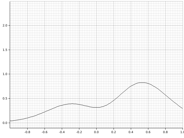
To start off with, take a function like so:

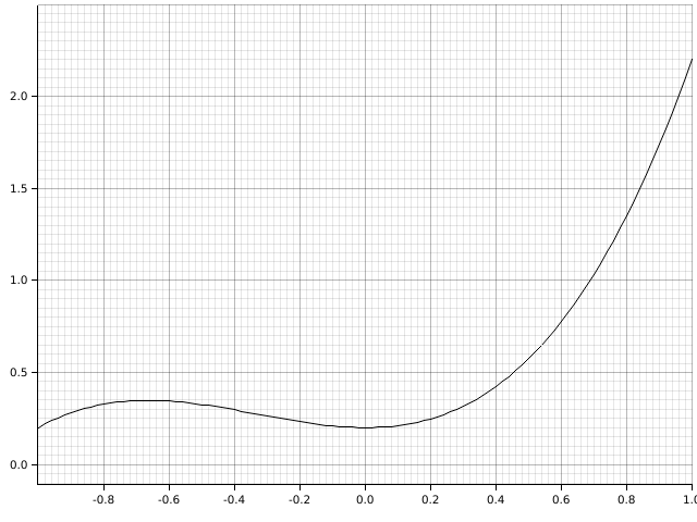
To find the area under the curve, there are some simple solutions. Two easy ones are the right- and left-rectangle rules:

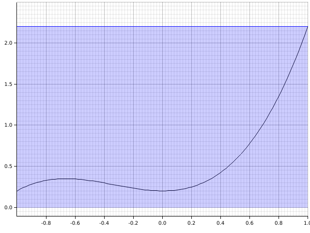
Mathematically, this becomes $$\int_a^b f(x)\,\mathrm{d}x \approx (b - a)f(b)$$ and $$\int_a^b f(x)\,\mathrm{d}x \approx (b - a)f(a) .$$

A better approach is to use the trapezoidal rule:

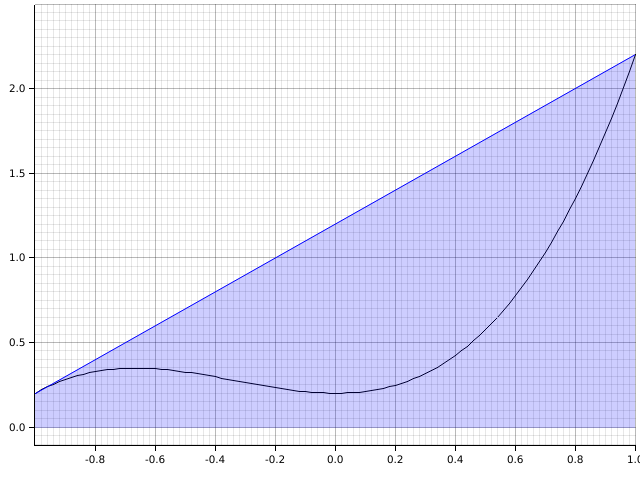
Mathematically, this is $$\int_a^b f(x)\,\mathrm{d}x \approx \frac{b - a}{2}\left(f(a) + f(b)\right) .$$ There is also Simpson’s rule, which uses an approximating parabola instead.

An easy way to improve accuracy is to break the interval up into smaller subintervals, turning a rule into a composite rule like so:

Mathematically, the composite trapezoidal rule is with step size $h$ is: $$\int_a^b f(x)\,\mathrm{d}x \approx \frac{h}{2}\left(f(a) + f(b)\right) + h\sum_1^{n-1} f(a + nh) .$$ This takes the form because each intermediate step is part of two trapezoids, the left trapezoid and the right trapezoid, canceling out the half. This rule is easily interleaved to use in adaptive quadrature. To half the step size, you can half the current integral value and then add in points half way between each of the current points multiplied by the halved step size.

Another approach to adaptive quadrature is to use Simpson’s rule. The range can be split into two, using Simpson’s rule on both the full range and each half. If the desired error is not met, each side of the range can be further subdivided. This concentrates calculations on the interesting bits of the integrand. bacon-sci has a function implementing this adaptive Simpson’s rule.

Generally, Simpson’s rule is better than the trapezoidal rule; however, it turns out that the trapezoidal rule is particularly good when the integrand decays double exponentially towards the end points (that is, decays as fast as $\exp(\exp(x))$ ). Taking advantage of this, we can do a variable substitution to integrate over the interval $[-1, 1]$ (Any two-sided closed interval can be changed to this one using another simple change of variable). A good change of variable to choose is $$x = \tanh\left(\frac{\pi}{2}\sinh t\right),$$ using hyperbolic trig functions. This changes the interval to $(-\infty, \infty)$ , pushing the end points out, so this gives an integration technique not sensitive to end point behavior. In the future, bacon-sci could use this to make integration functions where one or both endpoints have a singularity in the integrand. This change of variable changes the integral to $$\int_{-1}^1 f(x)\,\mathrm{d}x \approx \sum_{-\infty}^\infty w_k f(x_k),$$ where $$x_k = \tanh\left(\frac{\pi}{2}\sinh kh \right)$$ and $$w_k = \frac{\frac{h}{2}\pi \cosh kh}{\cosh^2\left(\frac{\pi}{2}\sinh kh\right)} .$$ This evaluates the transformed integral using the trapezoidal rule. Since the decay is double exponential, the limits on the sum can be made finite without much loss of precision. In bacon-sci, the sum is done from -3 to 3, which is correct within $1 \times 10^{-12}$ . 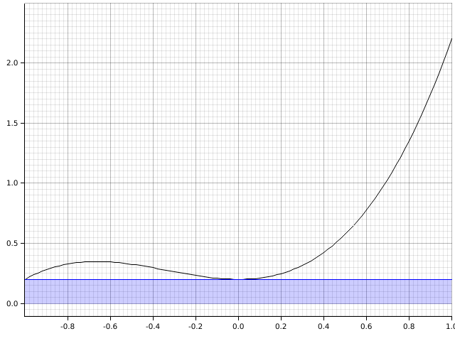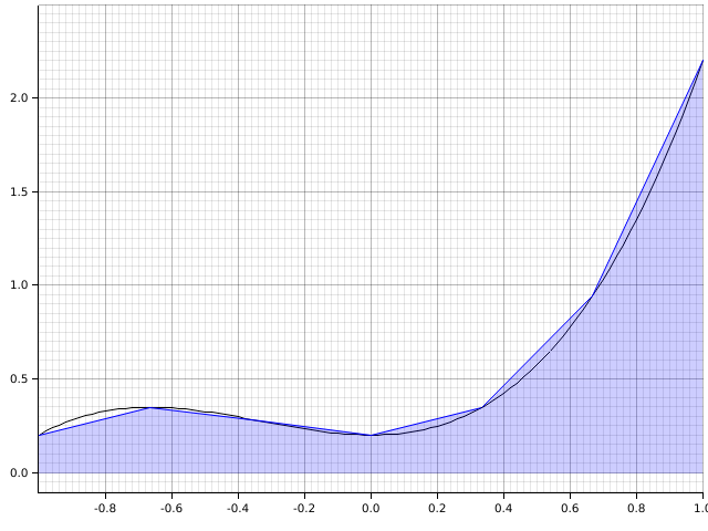For example, the transformed function from before looks like:

This method is called Tanh-Sinh integration. The weights and evaluation points are precomputed and stored in a lookup table. The trapezoidal rule is interlaced to compute the integral to a given precision. bacon-sci takes its implementation of Tanh-Sinh integration specifically from the quadrature crate, with attribution (quadrature is BSD licensed).

Tanh-Sinh quadrature is implemented as bacon_sci::integrate::integrate. Adaptive Simpson’s rule is bacon_sci::integrate::integrate_simpson. There is a fixed integration technique called Romberg integration implemented as bacon_sci::integrate::integrate_fixed.

Gaussian Integration

In the previous section, all of the integration rules used equally-spaced points. What if you could choose points spaced optimally for the integrand? Well, Gaussian integration does just that: it optimally spaces points so that the highest degree polynomial possible as an integrand is perfectly calculated.

Much like the section on special polynomials, Gaussian integration rules are determined by an interval and a weighting function. In general, the question is, what are the optimal points to evaluate to numerically integrate: $$\int_a^b f(x) w(x) \,\mathrm{d}x ?$$ As it turns out, the optimal $n$ points are the zeros of the $nth$ classical orthogonal polynomial on the interval $[a,b]$ with weighting function $w(x)$ as defined in the Special Polynomials section.

For general purpose integrals, the best interval is, like in Tanh-Sinh quadrature, $[-1,1]$ . This becomes Gaussian-Legendre quadrature. You can also integrate over $[0,\infty)$ with Gaussian-Laguerre quadrature and $(-\infty,\infty)$ with Gaussian-Hermite quadrature using the most natural weighting functions. In addition, bacon-sci provides both kinds of Chebyshev-Guassian quadrature. All of these integration functions can be done within a specified tolerance. Furthermore, all of the weighting function and polynomial zero evaluations are done ahead of time and stored in a table at compile-time. This is cool, but the best general purpose integration scheme is still Tanh-Sinh quadrature.

All Gaussian integration techniques discussed here are implemented under bacon_sci::integrate.

What’s Next?

There is much more to be added to bacon-sci. For example, many special functions can be added. Integration can be extended to integrate with end point singularities. Furthermore, I want to add statistics to bacon-sci. Distributions are already covered by rand_distr, but PDFs and CDFs can be added, as well as descriptive statistics. The next chapter in my numerical analysis book is optimization, so data fitting to a model using least-squares regression is to come. Lastly, of course, is optimizing what is currently in use. My integration functions are already fast, and my initial value problem solvers have benchmarked to be faster than both peroxide and SciPy. Maybe I’ll have a follow up blog comparing performance.